THIS PROJECT IS UNDER THE NEXT PHILOSOPHICAL PRINCIPLES

1) CONSCIOUSNESS IS INFINITE. CONVERSELY THE INFINITE IS A FUNCTION AND PROPERTY OF THE CONSCIOUSNESSES.

2) BUT THE PHYSICAL MATERIAL WORLD IS FINITE.

3) THEREFORE MATHEMATICAL MODELS IN THEIR ONTOLOGY SHOULD CONTAIN ONLY FINITE ENTITIES AND SHOULD NOT INVOLVE THE INFINITE.

THIS PROJECT THEREFORE IS CREATING AGAIN THE BASIC OF MATHEMATICS AND ITS ONTOLOGY WITH NEW AXIOMS THAT DO NOT INVOLVE THE INFINITE AT ALL.

Our perception and experience of the reality, depends on the system of beliefs that we have. In mathematics, the system of spiritual beliefs is nothing else than the axioms of the axiomatic systems that we accept. The rest is the work of reasoning and acting.

The abstraction of the infinite seems sweet at the beginning as it reduces some complexity, in the definitions, but later on it turns out to be bitter, as it traps the mathematical minds in to a vast complexity irrelevant to real life applications.

Classical mathematics with the infinite have more complicated logical setting (infinite) and less degrees of freedom of actions in applications. Digital mathematics have simpler logical setting (finite) and more degrees of freedom in actions of applications

We must realize that by describing an axiomatic system for the formal logic (1st, 2nd and higher finite order ω) we are in the realm of meta-mathematics, when we apply this formal logic to other axiomatic mathematical theories that are the ordinary mathematics. In general the size of the meta-mathematics compared to the size of mathematics is very important. Here we have a distinction and relevant terminology:

1) Size_of(meta-mathematics)>>size_of(mathematics)=> spiritual axiomatic theories,
In such theories, the objective realm has no non-measurable many elements (from the point of view of logic and meta-mathematics) , that is there is no concept of "infinite-like"

2) Size_of(meta-mathematics)<<size_of(mathematics)=> material axiomatic theories.

In such theories, the objective realm may have non-measurable many elements, (from the point of view of logic and meta-mathematics) that is there may be a concept of "infinite-like"

From the above we realize that the traditional mathematics with the classical Cantorian, concept of infinite, were created from the perspective of material theories rather than spiritual theories.

The discrimination of meta-mathematics and mathematics is the basis of the TRUE CONCEPT OF INFINITE-like ,
which is nothing more than the comparison of two finite numbers that count the resources of
a) the meta-mathematical resources of reasoning and expressing/formulating and
b) the mathematical resources of representing an ontological model of reality. Thus truly the infinite-like concept is the comparison of the (finite) resources of Logic and finite resources of Ontology. When naively in traditional Cantorian mathematics we talk about the infinite in reality we would like to express that the Ontology contains too many objects to count, given our resources of reasoning (Logic) and formulating. But in traditional Cantorian mathematics the definition of infinite took a totally formulation, that its complications and problems we skip here with our different and true approach.

By default , when we introduce the Formal Logic , we also assume the axiomatic system of the (digital) natural numbers. This we may call THE META-MATHEMATICAL NATURAL NUMBERS OR LOGICAL NATURAL NUMBERS. This is really very important to understand.

It is very interesting to watch carefully how the counting abilities and resources of the ontology of the objective theory of an axiomatic system, intermingle and combine with the counting abilities of the meta-mathematics or Logic.

As an metaphor in computers, the data of a database are entities of the mathematical ontology, while the files of the code and the content of the RAM memory, the resources of Logic and metamathematics.

For example, in an axiomatic system of the natural numbers, withing the formal logic, we may compare the logical natural numbers (which are the meta mathematical natural numbers that serve to count the formulas, symbols, proofs etc) with the natural numbers of the objective theory or ONTOLLOGICAL NATURAL NUMBERS. Such a comparison is at first of course within the meta-mathematics., but we may project it to the objective theory and derive second ontological system of natural numbers which is a copy of the Logical natural numbers.
Then we may have a simple definition of the infinite-like concept or materialitsticality of the ontology of it:
If for any logical natural number there is a greater ontological natural number, we say that the ontological natural numbers are INFINITE-like.
Notice that from the meta-mathematical point if view both the systems of Logical and ontological natural numbers are finite.

When a formal logical axiomatic system of natural numbers is infinite-like then an axiom like that of PEANO is necessary, Otherwise if the ontological natural numbers are finite it is not necessary, as it is possible within the utilized formal logic to derive a finite length proof of it. But if the onlological natural numbers are infinite-like (in the above digital sense) then the logical natural numbers are not sufficient many to construct a proof, therefore an axiom like that of Peano is necessary.
We will make it more detailed, and formally clear in the next.

The corresponding situation with the metaphor of a computer (the formal logic being a a computer), is that the information we intent to produce or store, in the computer exceeds the memory resources. So this information is "infinite-like" for this computer. And a corresponding proof of the induction axiom (Peano) would correspond to a run-time complexity, beyond the available maximum computing time.

There are people who believe that the infinite has a kind of spirituality because it is not met in natural reality, while the finite is more materialistic as it is found in nature and thus less spiritual. There may be a kind of truth in some situations about it. But there are many more situations that using the infinite shows a kind of spiritual inadequacy , spiritual inexperience while using the finite proves higher spirituality and realism.
As a coincidence in the Greek language the word infinite is the word απειρο which besides the mathematical meaning of infinite has also the natural Greek language meaning of "lack of experience". There are people who believe that talking and expressing about higher layers of the mind, like Logic and meta-mathematics shows higher spirituality. And there is some truth in it. But there are also people who believe that talking at all about higher layers of the mind is a lack of spirituality, while silence and internal contemplation is spirituality. I do not want to insist in particular to any of the above perspectives. But I do believe strongly, that re-writing the basic mathematics (and meta-mathematics) with an ontology that is completely avoiding any concept of Cantorian infinite, is a civilization necessity and requires and proves higher spirituality and existential integrity compared to the classical mathematics of the infinite.
Historically the introduction of the infinite might have been the best solution at that time (end of 19th beginning of 20th century). But I believe not anymore and as time passes the more we would do better as scientists and mathematicians in a universe of mathematics that does not have any Cantorian infinite.
At older historic times, that the frequency (relevant to the spin of electrons protons etc) of the human bodies was lower, the correlation with the material reality was often prohibiting clear thinking and the abstraction of the infinite that was obviously non-realistic for physical reality, was keeping the thinking mind in to safe distance from the physical reality. But now the frequency of the human civilization is higher, and thinking mathematically in a more realistic way, for the physical reality, only with finite avoiding the infinite seem possible and desirable.

I do not want to eliminate or disregard the classical mathematics with the infinite. It would be unwise, as it contains the work of hundreds and thousands of fine mathematicians. But I want to point out that in too many cases of applications in the physical world, we need a more realistic system of mathematics that does not use the infinite.
The leading interpretation principles, so as to derive and re-produce results in digital mathematics from results in classical mathematics are

A) The countable infinite is interpreted as a too large finite number, that we cannot count with our resources of formal logic, and we do not have information of how large it is (that is why we may denote it by ω)

B) For larger than countable , cardinal or ordinal e.g. α,β , with α<β and ω<=α again we interpret them as too large finite numbers, that we cannot count with our resources of formal logic, or have information of how large they are, but we do have information that α<β and ω<=α.

What is important here is that, the Formal Logic is formulated within some digital natural numbers, therefore, they have a Size Ω(l), which determines the feasible length of Logical formulae, logical formal proofs etc.

When formal logic is applied e.g. in digital real numbers, or digital Holographic Euclidean geometry, the size Ω(l) of the formal logic, and resolution ordinal , of the digital real numbers and digital holographic euclidean geometry, is important to compare, because it defines the provability or not of propositions, like in Goedel theorems of classical infinitary formal logic. It is all a matter of logical formal writing and space time resources rather, that absolute restrictions of the abilities of the mind.

Internal-external logic

1.4 The 1^st order formal Logic in digital mathematics.

We follow here the exposition in lines parallels to the exposition of classical infinitary 1st order logic in wikipedia, except we never accept any infinite set of symbols or other logical entities , as in Digital mathematics there is not any ontology of infinite. Furthermore because of this some additional logical axioms are added, to handle the relative sizes of the finite resources of logic (meta-mathematics) and mathematics.

http://en.wikipedia.org/wiki/Formal_Logic
http://en.wikipedia.org/wiki/Propositional_calculus

http://en.wikipedia.org/wiki/First-order_logic

Introduction

Propositional calculus

In mathematical logic, a propositional calculus or logic (also calledsentential calculus or sentential logic) is a formal system in which formulas of a formal language may be interpreted to representpropositions. A system of inference rules and axioms allows certain formulas to be derived. These derived formulas are called theorems and may be interpreted to be true propositions. Such a constructed sequence of formulas is known as a derivation or proof and the last formula of the sequence is the theorem. The derivation may be interpreted as proof of the proposition represented by the theorem.

Usually in Truth-functional propositional logic, formulas are interpreted as having either a truth value of true or a truth value or/ false.Truth-functional propositional logic and systems isomorphic to it, are considered to be zeroth-order logic.

AXIOMS OF THE RELATIVE RESOURCES OF PROPOSITIONAL CALCULUS.

The involved system of digital natural numbers, and digital set theory, are such that if Ω(Ν), and Ω(S), are the upper bounds of the sizes of them , then Ω(Ν)<= Ω(S).
Furthermore, the sizes of the sets of symbols, terms, formulas , predicate symbols, AND LENGTH OF PROOFS, are not only finite , but also small compared to Ω(Ν)<= Ω(S). That is if ω(l) is their total size,m then it is assumed constants M, and k, such that for all the Logical axiomatic systems that we discuss, within the 1st order or 2nd order formal Logic ω(l)<M<M^k<Ω(Ν)<= Ω(S). While
ω(l), Ω(Ν)<= Ω(S), may be variable, M , k are assumed constant, for all these systems.

Terminology

In general terms, a calculus is a formal system that consists of a set of syntactic expressions (well-formed formulæ orwffs), a distinguished subset of these expressions (axioms), plus a set of formal rules that define a specific binary relation, intended to be interpreted to be logical equivalence, on the space of expressions.

When the formal system is intended to be a logical system, the expressions are meant to be interpreted to be statements, and the rules, known to be inference rules, are typically intended to be truth-preserving. In this setting, the rules (which may include axioms) can then be used to derive ("infer") formulæ representing true statements from given formulæ representing true statements.

The set of axioms may be empty, a nonempty finite set, a countably infinite set, or be given by axiom schemata. Aformal grammar recursively defines the expressions and well-formed formulæ (wffs) of the language. In addition asemantics may be given which defines truth and valuations (or interpretations).

The language of a propositional calculus consists of

a set of primitive symbols (Sets here are from the Digital set theory thus always finite and upper bounded), variously referred to be atomic formulae, placeholders, proposition letters, orvariables, and
a set of operator symbols Sets here are from the Digital set theory thus always finite and upper bounded), variously interpreted to be logical operators or logical connectives.

A well-formed formula (wff) is any atomic formula, or any formula that can be built up from atomic formulæ by means of operator symbols according to the rules of the grammar.

Mathematicians sometimes distinguish between propositional constants, propositional variables, and schemata. Propositional constants represent some particular proposition, while propositional variables range over the set of all atomic propositions. Schemata, however, range over all propositions. It is common to represent propositional constants by

A

B

, and

C

, propositional variables by

P

Q

, and

R

, and schematic letters are often Greek letters, most often

\varphi \,\!

\psi

, and

\chi

Basic concepts

The following outlines a standard propositional calculus. Many different formulations exist which are all more or less equivalent but differ in the details of

their language, that is, the particular collection of primitive symbols and operator symbols,
the set of Sets here are from the Digital set theory thus always finite and upper bounded) axioms, or distinguished formulae, and
the set of inference rules.

We may represent any given proposition with a letter which we call a propositional constant, analogous to representing a number by a letter in mathematics, for instance,

a = 5

. We require that all propositions have exactly one of two truth-values: true or false. To take an example, let

P

be the proposition that it is raining outside. This will be true if it is raining outside and false otherwise.

We then define truth-functional operators, beginning with negation. We write $\neg P$ to represent the negation of $P$ , which can be thought of to be the denial of $P$ . In the example above, $\neg P$ expresses that it is not raining outside, or by a more standard reading: "It is not the case that it is raining outside." When $P$ is true, $\neg P$ is false; and when $P$ is false, $\neg P$ is true. $\neg \neg P$ always has the same truth-value as $P$ .
Conjunction is a truth-functional connective which forms a proposition out of two simpler propositions, for example, and . The conjunction of and is written , and expresses that each are true. We read for " and ". For any two propositions, there are four possible assignments of truth values:
1. $P$ is true and $Q$ is true
2. $P$ is true and $Q$ is false
3. $P$ is false and $Q$ is true
4. $P$ is false and $Q$ is false

The conjunction of

P

and

Q

is true in case 1 and is false otherwise. Where

P

is the proposition that it is raining outside and

Q

is the proposition that a cold-front is over Kansas,

P \and Q

is true when it is raining outside and there is a cold-front over Kansas. If it is not raining outside, then

P \and Q

is false; and if there is no cold-front over Kansas, then

P \and Q

is false.

Disjunction resembles conjunction in that it forms a proposition out of two simpler propositions. We write it $P \vee Q$ , and it is read " $P$ or $Q$ ". It expresses that either $P$ or $Q$ is true. Thus, in the cases listed above, the disjunction of $P$ and $Q$ is true in all cases except 4. Using the example above, the disjunction expresses that it is either raining outside or there is a cold front over Kansas. (Note, this use of disjunction is supposed to resemble the use of the English word "or". However, it is most like the English inclusive "or", which can be used to express the truth of at least one of two propositions. It is not like the English exclusive "or", which expresses the truth of exactly one of two propositions. That is to say, the exclusive "or" is false when both $P$ and $Q$ are true (case 1). An example of the exclusive or is: You may have a bagel or a pastry, but not both. Often in natural language, given the appropriate context, the addendum "but not both" is omitted but implied. In mathematics, however, "or" is always inclusive or; if exclusive or is meant it will be specified, possibly by "xor".)
Material conditional also joins two simpler propositions, and we write $P \rightarrow Q$ , which is read "if $P$ then $Q$ ". The proposition to the left of the arrow is called the antecedent and the proposition to the right is called the consequent. (There is no such designation for conjunction or disjunction, since they are commutative operations.) It expresses that $Q$ is true whenever $P$ is true. Thus it is true in every case above except case 2, because this is the only case when $P$ is true but $Q$ is not. Using the example, if $P$ then $Q$ expresses that if it is raining outside then there is a cold-front over Kansas. The material conditional is often confused with physical causation. The material conditional, however, only relates two propositions by their truth-values—which is not the relation of cause and effect. It is contentious in the literature whether the material implication represents logical causation.
Biconditional joins two simpler propositions, and we write $P \leftrightarrow Q$ , which is read " $P$ if and only if $Q$ ". It expresses that $P$ and $Q$ have the same truth-value, thus $P$ if and only if $Q$ is true in cases 1 and 4, and false otherwise.

It is extremely helpful to look at the truth tables for these different operators, as well as the method of analytic tableaux.

Closure under operations

Propositional logic is closed under truth-functional connectives. That is to say, for any proposition

\varphi \,\!

\neg \varphi \,\!

is also a proposition. Likewise, for any propositions

\varphi \,\!

and

\psi \,\!

\varphi \and \psi \,\!

is a proposition, and similarly for disjunction, conditional, and biconditional. This implies that, for instance,

P \and Q

is a proposition, and so it can be conjoined with another proposition. In order to represent this, we need to use parentheses to indicate which proposition is conjoined with which. For instance,

P \and Q \and R

is not a well-formed formula, because we do not know if we are conjoining

P \and Q

with

R

or if we are conjoining

P

with

Q \and R

. Thus we must write either

(P \and Q) \and R

to represent the former, or

P \and (Q \and R)

to represent the latter. By evaluating the truth conditions, we see that both expressions have the same truth conditions (will be true in the same cases), and moreover that any proposition formed by arbitrary conjunctions will have the same truth conditions, regardless of the location of the parentheses. This means that conjunction is associative, however, one should not assume that parentheses never serve a purpose. For instance, the sentence

P \and (Q \vee R)

does not have the same truth conditions of

(P \and Q) \vee R

, so they are different sentences distinguished only by the parentheses. One can verify this by the truth-table method referenced above.

Note: For any arbitrary small number (in digital natural numbers) of propositional constants, we can form a finite number of cases which list their possible truth-values. A simple way to generate this is by truth-tables, in which one writes

P

Q

, …,

Z

for any list of

k

propositional constants—that is to say, any list of propositional constants with

k

entries. Below this list, one writes

2^k

rows, and below

P

one fills in the first half of the rows with true (or T) and the second half with false (or F). Below

Q

one fills in one-quarter of the rows with T, then one-quarter with F, then one-quarter with T and the last quarter with F. The next column alternates between true and false for each eighth of the rows, then sixteenths, and so on, until the last propositional constant varies between T and F for each row. This will give a complete listing of cases or truth-value assignments possible for those propositional constants.

Argument

The propositional calculus then defines an argument to be a (finite always) set (of digital sets theory) of propositions. A valid argument is a set of propositions, the last of which follows from—or is implied by—the rest. All other arguments are invalid. The simplest valid argument is modus ponens, one instance of which is the following set of propositions:

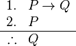
\begin{array}{rl} 1. & P \rightarrow Q \\ 2. & P \\ \hline \therefore & Q \end{array}

This is a set of three propositions, each line is a proposition, and the last follows from the rest. The first two lines are called premises, and the last line the conclusion. We say that any proposition

C

follows from any set of propositions

(P_1, ..., P_n)

, if

C

must be true whenever every member of the set

(P_1, ..., P_n)

is true. In the argument above, for any

P

and

Q

, whenever

P \rightarrow Q

and

P

are true, necessarily

Q

is true. Notice that, when

P

is true, we cannot consider cases 3 and 4 (from the truth table). When

P \rightarrow Q

is true, we cannot consider case 2. This leaves only case 1, in which Q is also true. Thus Q is implied by the premises.

This generalizes schematically. Thus, where

\varphi \,\!

and

\psi

may be any propositions at all,

\begin{array}{rl} 1. & \varphi \rightarrow \psi \\ 2. & \varphi \\ \hline \therefore & \psi \end{array}

Other argument forms are convenient, but not necessary. Given a complete set of axioms (see below for one such set), modus ponens is sufficient to prove all other argument forms in propositional logic, thus they may be considered to be a derivative. Note, this is not true of the extension of propositional logic to other logics like first-order logic. First-order logic requires at least one additional rule of inference in order to obtain completeness.

The significance of argument in formal logic is that one may obtain new truths from established truths. In the first example above, given the two premises, the truth of

Q

is not yet known or stated. After the argument is made,

Q

is deduced. In this way, we define a deduction system to be a set of all propositions that may be deduced from another set of propositions. For instance, given the set of propositions

A = \{ P \or Q, \neg Q \and R, (P \or Q) \rightarrow R \}

, we can define a deduction system,

\Gamma

, which is the set of all propositions which follow from

A

. Reiteration is always assumed, so

P \or Q, \neg Q \and R, (P \or Q) \rightarrow R \in \Gamma

. Also, from the first element of

A

, last element, as well as modus ponens,

R

is a consequence, and so

R \in \Gamma

. Because we have not included sufficiently complete axioms, though, nothing else may be deduced. Thus, even though most deduction systems studied in propositional logic are able to deduce

(P \or Q) \leftrightarrow (\neg P \rightarrow Q)

, this one is too weak to prove such a proposition.

Generic description of a propositional calculus

A propositional calculus is a formal system

\mathcal{L} = \mathcal{L} \left( \Alpha,\ \Omega,\ \Zeta,\ \Iota \right)

, where:

The alpha set $\Alpha$ is a finite set of elements called proposition symbols or propositional variables. Syntactically speaking, these are the most basic elements of the formal language $\mathcal{L}$ , otherwise referred to as atomic formulæor terminal elements. In the examples to follow, the elements of $\Alpha$ are typically the letters $p$ , $q$ , $r$ , and so on.

The omega set $\Omega$ is a finite set of elements called operator symbols or logical connectives. The set $\Omega$ ispartitioned into disjoint subsets as follows:

\Omega = \Omega_0 \cup \Omega_1 \cup \ldots \cup \Omega_j \cup \ldots \cup \Omega_m.

In this partition,

\Omega_j

is the set of operator symbols of arity

j

In the more familiar propositional calculi,

\Omega

is typically partitioned as follows:

\Omega_1 = \{ \lnot \},

\Omega_2 \subseteq \{ \land, \lor, \rightarrow, \leftrightarrow \}.

A frequently adopted convention treats the constant logical values as operators of arity zero, thus:

\Omega_0 = \{ 0, 1 \}.\,\!

Some writers use the tilde (~), or N, instead of

\neg

; and some use the ampersand (&), the prefixed K, or

\cdot

instead of

\wedge

. Notation varies even more for the set of logical values, with symbols like {false, true}, {F, T}, or

\{ \bot, \top \}

all being seen in various contexts instead of {0, 1}.

The zeta set $\Zeta$ is a finite set of transformation rules that are called inference rules when they acquire logical applications.

The iota set $\Iota$ is a finite set of initial points that are called axioms when they receive logical interpretations.

The language of

\mathcal{L}

, also known as its set of formulæ, well-formed formulas or wffs, is a finite set of digital set t theory, inductively defined by the following rules:

Base: Any element of the alpha set $\Alpha$ is a formula of $\mathcal{L}$ .
If $p_1, p_2, \ldots, p_j$ are formulæ and $f$ is in $\Omega_j$ , then $\left( f(p_1, p_2, \ldots, p_j) \right)$ is a formula.
Closed: Nothing else is a formula of $\mathcal{L}$ .

Repeated applications of these rules permits the construction of complex formulæ. For example:

By rule 1, $p$ is a formula.
By rule 2, $\neg p$ is a formula.
By rule 1, $q$ is a formula.
By rule 2, $( \neg p \lor q )$ is a formula.

Example 1. Simple axiom system

Let

\mathcal{L}_1 = \mathcal{L}(\Alpha,\Omega,\Zeta,\Iota)

, where

\Alpha

\Omega

\Zeta

\Iota

are defined as follows:

The alpha set $\Alpha$ , is a finite set of symbols that is large enough to supply the needs of a given discussion, for example:

\Alpha = \{p, q, r, s, t, u \}.\,\!

Of the three connectives for conjunction, disjunction, and implication ( $\wedge$ , $\lor$ , and $\rightarrow$ ), one can be taken as primitive and the other two can be defined in terms of it and negation ( $\neg$ ).^[8] Indeed, all of the logical connectives can be defined in terms of a sole sufficient operator. The biconditional ( $\leftrightarrow$ ) can of course be defined in terms of conjunction and implication, with $a \leftrightarrow b$ defined as $(a \to b) \land (b \to a)$ .

Adopting negation and implication as the two primitive operations of a propositional calculus is tantamount to having the omega set

\Omega = \Omega_1 \cup \Omega_2

partition as follows:

\Omega_1 = \{ \lnot \},

\Omega_2 = \{ \rightarrow \}.

An axiom system discovered by Jan Łukasiewicz formulates a propositional calculus in this language as follows. The axioms are all substitution instances of:

$(p \to (q \to p))$

$((p \to (q \to r)) \to ((p \to q) \to (p \to r)))$

$((\neg p \to \neg q) \to (q \to p))$

The rule of inference is modus ponens (i.e., from $p$ and $(p \to q)$ , infer $q$ ). Then $a \lor b$ is defined as $\neg a \to b$ , and $a \land b$ is defined as $\neg(a \to \neg b)$ .

Example 2. Natural deduction system

Let

\mathcal{L}_2 = \mathcal{L}(\Alpha, \Omega, \Zeta, \Iota)

, where

\Alpha

\Omega

\Zeta

\Iota

are defined as follows:

The alpha set $\Alpha$ , is a finite set of symbols that is large enough to supply the needs of a given discussion, for example:
$\Alpha = \{p, q, r, s, t, u \}.\,\!$
The omega set $\Omega = \Omega_1 \cup \Omega_2$ partitions as follows:
$\Omega_1 = \{ \lnot \},$
$\Omega_2 = \{ \land, \lor, \rightarrow, \leftrightarrow \}.$

In the following example of a propositional calculus, the transformation rules are intended to be interpreted as the inference rules of a so-called natural deduction system. The particular system presented here has no initial points, which means that its interpretation for logical applications derives its theorems from an empty axiom set.

The set of initial points is empty, that is, $\Iota = \varnothing$ .
The set of transformation rules, $\Zeta$ , is described as follows:

Our propositional calculus has ten inference rules. These rules allow us to derive other true formulae given a set of formulae that are assumed to be true. The first nine simply state that we can infer certain wffs from other wffs. The last rule however uses hypothetical reasoning in the sense that in the premise of the rule we temporarily assume an (unproven) hypothesis to be part of the set of inferred formulae to see if we can infer a certain other formula. Since the first nine rules don't do this they are usually described as non-hypothetical rules, and the last one as ahypothetical rule.

In describing the transformation rules, we may introduce a metalanguage symbol

\vdash

. It is basically a convenient shorthand for saying "infer that". The format is

\Gamma \vdash \psi

, in which

\Gamma

is a (possibly empty) set of formulae called premises, and

\psi

is a formula called conclusion. The transformation rule

\Gamma \vdash \psi

means that if every proposition in

\Gamma

is a theorem (or has the same truth value as the axioms), then

\psi

is also a theorem. Note that considering the following rule Conjunction introduction, we will know whenever

\Gamma

has more than one formula, we can always safely reduce it into one formula using conjunction. So for short, from that time on we may represent

\Gamma

as one formula instead of a set. Another omission for convenience is when

\Gamma

is an empty set, in which case

\Gamma

may not appear.

Negation introduction: From $(p \to q)$ and $(p \to \neg q)$ , infer $\neg p$ .; That is, $\{ (p \to q), (p \to \neg q) \} \vdash \neg p$ .
Negation elimination: From $\neg p$ , infer $(p \to r)$ .; That is, $\{ \neg p \} \vdash (p \to r)$ .
Double negative elimination: From $\neg \neg p$ , infer $p$ .; That is, $\neg \neg p \vdash p$ .
Conjunction introduction: From $p$ and $q$ , infer $(p \land q)$ .; That is, $\{ p, q \} \vdash (p \land q)$ .
Conjunction elimination: From $(p \land q)$ , infer $p$ .; From $(p \land q)$ , infer $q$ .; That is, $(p \land q) \vdash p$ and $(p \land q) \vdash q$ .
Disjunction introduction: From $p$ , infer $(p \lor q)$ .; From $q$ , infer $(p \lor q)$ .; That is, $p \vdash (p \lor q)$ and $q \vdash (p \lor q)$ .
Disjunction elimination: From $(p \lor q)$ and $(p \to r)$ and $(q \to r)$ , infer $r$ .; That is, $\{p \lor q, p \to r, q \to r\} \vdash r$ .
Biconditional introduction: From $(p \to q)$ and $(q \to p)$ , infer $(p \leftrightarrow q)$ .; That is, $\{p \to q, q \to p\} \vdash (p \leftrightarrow q)$ .
Biconditional elimination: From $(p \leftrightarrow q)$ , infer $(p \to q)$ .; From $(p \leftrightarrow q)$ , infer $(q \to p)$ .; That is, $(p \leftrightarrow q) \vdash (p \to q)$ and $(p \leftrightarrow q) \vdash (q \to p)$ .
Modus ponens (conditional elimination): From $p$ and $(p \to q)$ , infer $q$ .; That is, $\{ p, p \to q\} \vdash q$ .
Conditional proof (conditional introduction): From [accepting $p$ allows a proof of $q$ ], infer $(p \to q)$ .; That is, $(p \vdash q) \vdash (p \to q)$ .

Basic and derived argument forms

Basic and Derived Argument Forms
Name	Sequent	Description
Modus Ponens	$((p \to q) \land p) \vdash q$	If $p$ then $q$ ; $p$ ; therefore $q$
Modus Tollens	$((p \to q) \land \neg q) \vdash \neg p$	If $p$ then $q$ ; not $q$ ; therefore not $p$
Hypothetical Syllogism	$((p \to q) \land (q \to r)) \vdash (p \to r)$	If $p$ then $q$ ; if $q$ then $r$ ; therefore, if $p$ then $r$
Disjunctive Syllogism	$((p \lor q) \land \neg p) \vdash q$	Either $p$ or $q$ , or both; not $p$ ; therefore, $q$
Constructive Dilemma	$((p \to q) \land (r \to s) \land (p \lor r)) \vdash (q \lor s)$	If $p$ then $q$ ; and if $r$ then $s$ ; but $p$ or $r$ ; therefore $q$ or $s$
Destructive Dilemma	$((p \to q) \land (r \to s) \land(\neg q \lor \neg s)) \vdash (\neg p \lor \neg r)$	If $p$ then $q$ ; and if $r$ then $s$ ; but not $q$ or not $s$ ; therefore not $p$ or not $r$
Bidirectional Dilemma	$((p \to q) \land (r \to s) \land(p \lor \neg s)) \vdash (q \lor \neg r)$	If $p$ then $q$ ; and if $r$ then $s$ ; but $p$ or not $s$ ; therefore $q$ or not $r$
Simplification	$(p \land q) \vdash p$	$p$ and $q$ are true; therefore $p$ is true
Conjunction	$p, q \vdash (p \land q)$	$p$ and $q$ are true separately; therefore they are true conjointly
Addition	$p \vdash (p \lor q)$	$p$ is true; therefore the disjunction ( $p$ or $q$ ) is true
Composition	$((p \to q) \land (p \to r)) \vdash (p \to (q \land r))$	If $p$ then $q$ ; and if $p$ then $r$ ; therefore if $p$ is true then $q$ and $r$ are true
De Morgan's Theorem(1)	$\neg (p \land q) \vdash (\neg p \lor \neg q)$	The negation of ( $p$ and $q$ ) is equiv. to (not $p$ or not $q$ )
De Morgan's Theorem(2)	$\neg (p \lor q) \vdash (\neg p \land \neg q)$	The negation of ( $p$ or $q$ ) is equiv. to (not $p$ and not $q$ )
Commutation (1)	$(p \lor q) \vdash (q \lor p)$	( $p$ or $q$ ) is equiv. to ( $q$ or $p$ )
Commutation (2)	$(p \land q) \vdash (q \land p)$	( $p$ and $q$ ) is equiv. to ( $q$ and $p$ )
Commutation (3)	$(p \leftrightarrow q) \vdash (q \leftrightarrow p)$	( $p$ is equiv. to $q$ ) is equiv. to ( $q$ is equiv. to $p$ )
Association (1)	$(p \lor (q \lor r)) \vdash ((p \lor q) \lor r)$	$p$ or ( $q$ or $r$ ) is equiv. to ( $p$ or $q$ ) or $r$
Association (2)	$(p \land (q \land r)) \vdash ((p \land q) \land r)$	$p$ and ( $q$ and $r$ ) is equiv. to ( $p$ and $q$ ) and $r$
Distribution (1)	$(p \land (q \lor r)) \vdash ((p \land q) \lor (p \land r))$	$p$ and ( $q$ or $r$ ) is equiv. to ( $p$ and $q$ ) or ( $p$ and $r$ )
Distribution (2)	$(p \lor (q \land r)) \vdash ((p \lor q) \land (p \lor r))$	$p$ or ( $q$ and $r$ ) is equiv. to ( $p$ or $q$ ) and ( $p$ or $r$ )
Double Negation	$p \vdash \neg \neg p$	$p$ is equivalent to the negation of not $p$
Transposition	$(p \to q) \vdash (\neg q \to \neg p)$	If $p$ then $q$ is equiv. to if not $q$ then not $p$
Material Implication	$(p \to q) \vdash (\neg p \lor q)$	If $p$ then $q$ is equiv. to not $p$ or $q$
Material Equivalence(1)	$(p \leftrightarrow q) \vdash ((p \to q) \land (q \to p))$	( $p$ iff $q$ ) is equiv. to (if $p$ is true then $q$ is true) and (if $q$ is true then $p$ is true)
Material Equivalence(2)	$(p \leftrightarrow q) \vdash ((p \land q) \lor (\neg p \land \neg q))$	( $p$ iff $q$ ) is equiv. to either ( $p$ and $q$ are true) or (both $p$ and $q$ are false)
Material Equivalence(3)	$(p \leftrightarrow q) \vdash ((p \lor \neg q) \land (\neg p \lor q))$	( $p$ iff $q$ ) is equiv to., both ( $p$ or not $q$ is true) and (not $p$ or $q$ is true)
Exportation^[9]	$((p \land q) \to r) \vdash (p \to (q \to r))$	from (if $p$ and $q$ are true then $r$ is true) we can prove (if $q$ is true then $r$ is true, if $p$ is true)
Importation	$(p \to (q \to r)) \vdash ((p \land q) \to r)$	If $p$ then (if $q$ then $r$ ) is equivalent to if $p$ and $q$ then $r$
Tautology (1)	$p \vdash (p \lor p)$	$p$ is true is equiv. to $p$ is true or $p$ is true
Tautology (2)	$p \vdash (p \land p)$	$p$ is true is equiv. to $p$ is true and $p$ is true
Tertium non datur (Law of Excluded Middle)	$\vdash (p \lor \neg p)$	$p$ or not $p$ is true
Law of Non-Contradiction	$\vdash \neg (p \land \neg p)$	$p$ and not $p$ is false, is a true statement

Proofs in propositional calculus

One of the main uses of a propositional calculus, when interpreted for logical applications, is to determine relations of logical equivalence between propositional formulæ. These relationships are determined by means of the available transformation rules, sequences of which are called derivations or proofs.

In the discussion to follow, a proof is presented as a FINITE sequence of numbered lines, with each line consisting of a single formula followed by a reason or justification for introducing that formula. Each premise of the argument, that is, an assumption introduced as an hypothesis of the argument, is listed at the beginning of the sequence and is marked as a "premise" in lieu of other justification. The conclusion is listed on the last line. A proof is complete if every line follows from the previous ones by the correct application of a transformation rule. (For a contrasting approach, see proof-trees).

Example of a proof

To be shown that $A \to A$ .

One possible proof of this (which, though valid, happens to contain more steps than are necessary) may be arranged as follows:

Example of a Proof
Number	Formula	Reason
1	$A\,\!$	premise
2	$A \lor A$	From (1) by disjunction introduction
3	$(A \lor A) \land A$	From (1) and (2) by conjunction introduction
4	$A\,\!$	From (3) by conjunction elimination
5	$A \vdash A$	Summary of (1) through (4)
6	$\vdash A \to A$	From (5) by conditional proof

Interpret

A \vdash A

as "Assuming

A

, infer

A

". Read

\vdash A \to A

as "Assuming nothing, infer that

A

implies

A

", or "It is a tautology that

A

implies

A

", or "It is always true that

A

implies

A

Soundness and completeness of the rules

The crucial properties of this set of rules are that they are sound and complete. Informally this means that the rules are correct and that no other rules are required. These claims can be made more formal as follows.

We define a truth assignment as a function that maps propositional variables to true or false. Informally such a truth assignment can be understood as the description of a possible state of affairs (or possible world) where certain statements are true and others are not. The semantics of formulae can then be formalized by defining for which "state of affairs" they are considered to be true, which is what is done by the following definition.

We define when such a truth assignment

A \,

satisfies a certain wff with the following rules:

$A \,$ satisfies the propositional variable $P \,$ if and only if $A(P) = \text{true} \,$
$A \,$ satisfies $\neg \phi \,$ if and only if $A \,$ does not satisfy $\phi \,$
$A \,$ satisfies $(\phi \land \psi) \,$ if and only if $A \,$ satisfies both $\phi \,$ and $\psi \,$
$A \,$ satisfies $(\phi \lor \psi) \,$ if and only if $A \,$ satisfies at least one of either $\phi \,$ or $\psi \,$
$A \,$ satisfies $(\phi \to \psi) \,$ if and only if it is not the case that $A \,$ satisfies $\phi \,$ but not $\psi \,$
$A \,$ satisfies $(\phi \leftrightarrow \psi) \,$ if and only if $A \,$ satisfies both $\phi \,$ and $\psi \,$ or satisfies neither one of them

With this definition we can now formalize what it means for a formula

\phi \,

to be implied by a certain set

S \,

of formulae. Informally this is true if in all worlds that are possible given the set of formulae

S \,

the formula

\phi \,

also holds. This leads to the following formal definition: We say that a set

S \,

of wffs semantically entails (or implies) a certain wff

\phi \,

if all truth assignments that satisfy all the formulae in

S \,

also satisfy

\phi \,.

Finally we define syntactical entailment such that

\phi \,

is syntactically entailed by

S \,

if and only if we can derive it with the inference rules that were presented above in a finite number of steps. This allows us to formulate exactly what it means for the set of inference rules to be sound and complete:

Soundness: If the set of wffs $S \,$ syntactically entails wff $\phi \,$ then $S \,$ semantically entails $\phi \,$
Completeness: If the set of wffs $S \,$ semantically entails wff $\phi \,$ then $S \,$ syntactically entails $\phi \,$

For the above set of rules this is indeed the case.

Sketch of a soundness proof

(For most logical systems, this is the comparatively "simple" direction of proof)

Notational conventions: Let

G

be a variable ranging over sets of sentences. Let

A

B

, and

C

range over sentences. For "

G

syntactically entails

A

" we write "

G

proves

A

". For "

G

semantically entails

A

" we write "

G

implies

A

We want to show: (

A

)(

G

)(if

G

proves

A

, then

G

implies

A

We note that "

G

proves

A

" has an inductive definition, and that gives us the immediate resources for demonstrating claims of the form "If

G

proves

A

, then ...". So our proof proceeds by induction.

Basis. Show: If $A$ is a member of $G$ , then $G$ implies $A$ .
Basis. Show: If $A$ is an axiom, then $G$ implies $A$ .
Inductive step (induction on , the length of the proof):
1. Assume for arbitrary $G$ and $A$ that if $G$ proves $A$ in $n$ or fewer steps, then $G$ implies $A$ .
2. For each possible application of a rule of inference at step $n+1$ , leading to a new theorem $B$ , show that $G$ implies $B$ .

Notice that Basis Step II can be omitted for natural deduction systems because they have no axioms. When used, Step II involves showing that each of the axioms is a (semantic) logical truth.

The Basis steps demonstrate that the simplest provable sentences from

G

are also implied by

G

, for any

G

. (The proof is simple, since the semantic fact that a set implies any of its members, is also trivial.) The Inductive step will systematically cover all the further sentences that might be provable—by considering each case where we might reach a logical conclusion using an inference rule—and shows that if a new sentence is provable, it is also logically implied. (For example, we might have a rule telling us that from "

A

" we can derive "

A

B

". In III.a We assume that if

A

is provable it is implied. We also know that if

A

is provable then "

A

B

" is provable. We have to show that then "

A

B

" too is implied. We do so by appeal to the semantic definition and the assumption we just made.

A

is provable from

G

, we assume. So it is also implied by

G

. So any semantic valuation making all of

G

true makes

A

true. But any valuation making

A

true makes "

A

B

" true, by the defined semantics for "or". So any valuation which makes all of

G

true makes "

A

B

" true. So "

A

B

" is implied.) Generally, the Inductive step will consist of a lengthy but simple case-by-case analysis of all the rules of inference, showing that each "preserves" semantic implication.

By the definition of provability, there are no sentences provable other than by being a member of

G

, an axiom, or following by a rule; so if all of those are semantically implied, the deduction calculus is sound.

Sketch of completeness proof

(This is usually the much harder direction of proof.)

We adopt the same notational conventions as above.

We want to show: If

G

implies

A

, then

G

proves

A

. We proceed by contraposition: We show instead that if

G

doesnot prove

A

then

G

does not imply

A

$G$ does not prove $A$ . (Assumption)
If does not prove , then we can construct an (infinite) "Maximal Set", , which is a superset of and which also does not prove .
1. Place an "ordering" on all the sentences in the language (e.g., shortest first, and equally long ones in extended alphabetical ordering), and number them $E_1$ , $E_2$ , …(here 1,2,3 etc are digital natural numbers)
2. Define a series of sets (, , …) inductively:
  1. $G_0 = G$
  2. If $G_k \cup \{ E_{k+1} \}$ proves $A$ , then $G_{k+1} = G_k$
  3. If $G_k \cup \{ E_{k+1} \}$ does not prove $A$ , then $G_{k+1} = G_k \cup \{ E_{k+1} \}$
3. Define $G^*$ as the union of all the $G_n$ . (That is, $G^*$ is the set of all the sentences that are in any $G_n$ .)
4. It can be easily shown that
  1. $G^*$ contains (is a superset of) $G$ (by (b.i));
  2. $G^*$ does not prove $A$ (because if it proves $A$ then some sentence was added to some $G_n$ which caused it to prove ' $A$ ; but this was ruled out by definition); and
  3. $G^*$ is a "Maximal Set" (with respect to $A$ ): If any more sentences whatever were added to $G^*$ , it would prove $A$ . (Because if it were possible to add any more sentences, they should have been added when they were encountered during the construction of the $G_n$ , again by definition)
If $G^*$ is a Maximal Set (wrt $A$ ), then it is "truth-like". This means that it contains the sentence " $C$ " only if it does not contain the sentence not- $C$ ; If it contains " $C$ " and contains "If $C$ then $B$ " then it also contains " $B$ "; and so forth.
If $G^*$ is truth-like there is a " $G^*$ -Canonical" valuation of the language: one that makes every sentence in $G^*$ true and everything outside $G^*$ false while still obeying the laws of semantic composition in the language.
A $G^*$ -canonical valuation will make our original set $G$ all true, and make $A$ false.
If there is a valuation on which $G$ are true and $A$ is false, then $G$ does not (semantically) imply $A$ .

QED

Another outline for a completeness proof

If a formula is a tautology, then there is a truth table for it which shows that each valuation yields the value true for the formula. Consider such a valuation. By mathematical induction on the length of the subformulae, show that the truth or falsity of the subformula follows from the truth or falsity (as appropriate for the valuation) of each propositional variable in the subformula. Then combine the lines of the truth table together two at a time by using "(P is true implies S) implies ((P is false implies S) implies S)". Keep repeating this until all dependencies on propositional variables have been eliminated. The result is that we have proved the given tautology. Since every tautology is provable, the logic is complete.

Interpretation of a truth-functional propositional calculus

An interpretation of a truth-functional propositional calculus

\mathcal{P}

is an assignment to each propositional symbolof

\mathcal{P}

of one or the other (but not both) of the truth values truth (T) and falsity (F), and an assignment to theconnective symbols of

\mathcal{P}

of their usual truth-functional meanings. An interpretation of a truth-functional propositional calculus may also be expressed in terms of truth tables.

For

n

distinct propositional symbols there are

2^n

distinct possible interpretations. For any particular symbol

a

, for example, there are

2^1=2

possible interpretations:

$a$ is assigned T, or
$a$ is assigned F.

For the pair

a

b

there are

2^2=4

possible interpretations:

both are assigned T,
both are assigned F,
$a$ is assigned T and $b$ is assigned F, or
$a$ is assigned F and $b$ is assigned T.^[10]

Since

\mathcal{P}

has

\aleph_0

, that is, denumerably many propositional symbols, there are

2^{\aleph_0}=\mathfrak c

, and therefore uncountably many distinct possible interpretations of

\mathcal{P}

.^[10]

Interpretation of a sentence of truth-functional propositional logic

\phi\,\!

and

\psi

are formulae of

\mathcal{P}

and

\mathcal{I}

is an interpretation of

\mathcal{P}

then:

A sentence of propositional logic is true under an interpretation $\mathcal{I}$ iff $\mathcal{I}$ assigns the truth value T to that sentence. If a sentence is true under an interpretation, then that interpretation is called a model of that sentence.
$\phi\,\!$ is false under an interpretation $\mathcal{I}$ iff $\phi\,\!$ is not true under $\mathcal{I}$ .^[10]
A sentence of propositional logic is logically valid iff it is true under every interpretation

\models\phi

means that

\phi\,\!

is logically valid

A sentence $\psi$ of propositional logic is a semantic consequence of a sentence $\phi\,\!$ iff there is no interpretation under which $\phi\,\!$ is true and $\psi$ is false.
A sentence of propositional logic is consistent iff it is true under at least one interpretation. It is inconsistent if it is not consistent.

Some consequences of these definitions:

For any given interpretation a given formula is either true or false.^[10]
No formula is both true and false under the same interpretation.^[10]
$\phi\,\!$ is false for a given interpretation iff $\neg\phi$ is true for that interpretation; and $\phi\,\!$ is true under an interpretation iff $\neg\phi$ is false under that interpretation.^[10]
If $\phi\,\!$ and $(\phi \rightarrow \psi)$ are both true under a given interpretation, then $\psi$ is true under that interpretation.^[10]
If $\models_{\mathrm P}\phi$ and $\models_{\mathrm P}(\phi \rightarrow \psi)$ , then $\models_{\mathrm P}\psi$ .^[10]
$\neg\phi$ is true under $\mathcal{I}$ iff $\phi\,\!$ is not true under $\mathcal{I}$ .
$(\phi \rightarrow \psi)$ is true under $\mathcal{I}$ iff either $\phi\,\!$ is not true under $\mathcal{I}$ or $\psi$ is true under $\mathcal{I}$ .^[10]
A sentence $\psi$ of propositional logic is a semantic consequence of a sentence $\phi\,\!$ iff $(\phi \rightarrow \psi)$ is logically valid, that is, $\phi \models_{\mathrm P} \psi$ iff $\models_{\mathrm P}(\phi \rightarrow \psi)$ .^[10]

Alternative calculus

It is possible to define another version of propositional calculus, which defines most of the syntax of the logical operators by means of axioms, and which uses only one inference rule.

Axioms

Let

\phi\,\!

\chi

and

\psi

stand for well-formed formulæ. (The wffs themselves would not contain any Greek letters, but only capital Roman letters, connective operators, and parentheses.) Then the axioms are as follows:

Axioms
Name	Axiom Schema	Description
THEN-1	$\phi \to (\chi \to \phi)$	Add hypothesis $\chi$ , implication introduction
THEN-2	$(\phi \to (\chi \to \psi)) \to ((\phi \to \chi) \to (\phi \to \psi))$	Distribute hypothesis $\phi\,\!$ over implication
AND-1	$\phi \land \chi \to \phi$	Eliminate conjunction
AND-2	$\phi \land \chi \to \chi$
AND-3	$\phi \to (\chi \to (\phi \land \chi))$	Introduce conjunction
OR-1	$\phi \to \phi \lor \chi$	Introduce disjunction
OR-2	$\chi \to \phi \lor \chi$
OR-3	$(\phi \to \psi) \to ((\chi \to \psi) \to (\phi \lor \chi \to \psi))$	Eliminate disjunction
NOT-1	$(\phi \to \chi) \to ((\phi \to \neg \chi) \to \neg \phi)$	Introduce negation
NOT-2	$\phi \to (\neg \phi \to \chi)$	Eliminate negation
NOT-3	$\phi \lor \neg \phi$	Excluded middle, classical logic
IFF-1	$(\phi \leftrightarrow \chi) \to (\phi \to \chi)$	Eliminate equivalence
IFF-2	$(\phi \leftrightarrow \chi) \to (\chi \to \phi)$
IFF-3	$(\phi \to \chi) \to ((\chi \to \phi) \to (\phi \leftrightarrow \chi))$	Introduce equivalence

Axiom THEN-2 may be considered to be a "distributive property of implication with respect to implication."
Axioms AND-1 and AND-2 correspond to "conjunction elimination". The relation between AND-1 and AND-2 reflects the commutativity of the conjunction operator.
Axiom AND-3 corresponds to "conjunction introduction."
Axioms OR-1 and OR-2 correspond to "disjunction introduction." The relation between OR-1 and OR-2 reflects the commutativity of the disjunction operator.
Axiom NOT-1 corresponds to "reductio ad absurdum."
Axiom NOT-2 says that "anything can be deduced from a contradiction."
Axiom NOT-3 is called "tertium non datur" (Latin: "a third is not given") and reflects the semantic valuation of propositional formulae: a formula can have a truth-value of either true or false. There is no third truth-value, at least not in classical logic. Intuitionistic logicians do not accept the axiom NOT-3.

Inference rule

The inference rule is modus ponens:

\phi, \ \phi \rightarrow \chi \vdash \chi

Meta-inference rule

Let a demonstration be represented by a sequence, with hypotheses to the left of the turnstile and the conclusion to the right of the turnstile. Then the deduction theorem can be stated as follows:

If the sequence

\phi_1, \ \phi_2, \ ... , \ \phi_n, \ \chi \vdash \psi

has been demonstrated, then it is also possible to demonstrate the sequence

\phi_1, \ \phi_2, \ ..., \ \phi_n \vdash \chi \rightarrow \psi

This deduction theorem (DT) is not itself formulated with propositional calculus: it is not a theorem of propositional calculus, but a theorem about propositional calculus. In this sense, it is a meta-theorem, comparable to theorems about the soundness or completeness of propositional calculus.

On the other hand, DT is so useful for simplifying the syntactical proof process that it can be considered and used as another inference rule, accompanying modus ponens. In this sense, DT corresponds to the natural conditional proofinference rule which is part of the first version of propositional calculus introduced in this article.

The converse of DT is also valid:

If the sequence

\phi_1, \ \phi_2, \ ..., \ \phi_n \vdash \chi \rightarrow \psi

has been demonstrated, then it is also possible to demonstrate the sequence

\phi_1, \ \phi_2, \ ... , \ \phi_n, \ \chi \vdash \psi

in fact, the validity of the converse of DT is almost trivial compared to that of DT:

\phi_1, \ ... , \ \phi_n \vdash \chi \rightarrow \psi

then

\phi_1, \ ... , \ \phi_n, \ \chi \vdash \chi \rightarrow \psi

\phi_1, \ ... , \ \phi_n, \ \chi \vdash \chi

and from (1) and (2) can be deduced

\phi_1, \ ... , \ \phi_n, \ \chi \vdash \psi

by means of modus ponens, Q.E.D.

The converse of DT has powerful implications: it can be used to convert an axiom into an inference rule. For example, the axiom AND-1,

\vdash \phi \wedge \chi \rightarrow \phi

can be transformed by means of the converse of the deduction theorem into the inference rule

\phi \wedge \chi \vdash \phi

which is conjunction elimination, one of the ten inference rules used in the first version (in this article) of the propositional calculus.

Example of a proof

The following is an example of a (syntactical) demonstration, involving only axioms THEN-1 and THEN-2:

Prove:

A \rightarrow A

(Reflexivity of implication).

Proof:

$(A \rightarrow ((B \rightarrow A) \rightarrow A)) \rightarrow ((A \rightarrow (B \rightarrow A)) \rightarrow (A \rightarrow A))$
Axiom THEN-2 with $\phi = A\,\!$ , $\chi = B \rightarrow A$ , $\psi = A$
$A \rightarrow ((B \rightarrow A) \rightarrow A)$
Axiom THEN-1 with $\phi = A\,\!$ , $\chi = B \rightarrow A$
$(A \rightarrow (B \rightarrow A)) \rightarrow (A \rightarrow A)$
From (1) and (2) by modus ponens.
$A \rightarrow (B \rightarrow A)$
Axiom THEN-1 with $\phi = A\,\!$ , $\chi = B$
$A \rightarrow A$
From (3) and (4) by modus ponens.

The 1^st order formal Logic

Syntax

There are two key parts of first-order logic. The syntax determines which collections of symbols are legal expressions in first-order logic, while the semantics determine the meanings behind these expressions.

Alphabet

Unlike natural languages, such as English, the language of first-order logic is completely formal, so that it can be mechanically determined whether a given expression is legal. There are two key types of legal expressions: terms, which intuitively represent objects, and formulas, which intuitively express predicates that can be true or false. The terms and formulas of first-order logic are strings of symbols which together form the alphabet of the language. As with all formal languages, the nature of the symbols themselves is outside the scope of formal logic; they are often regarded simply as letters and punctuation symbols.

It is common to divide the symbols of the alphabet into logical symbols, which always have the same meaning, and non-logical symbols, whose meaning varies by interpretation. For example, the logical symbol

\land

always represents "and"; it is never interpreted as "or". On the other hand, a non-logical predicate symbol such as Phil(x) could be interpreted to mean "x is a philosopher", "x is a man named Philip", or any other unary predicate, depending on the interpretation at hand.

Logical symbols

There are several logical symbols in the alphabet, which vary by author but usually include:

The quantifier symbols ∀ and ∃
The logical connectives: ∧ for conjunction, ∨ for disjunction, → for implication, ↔ for biconditional, ¬ for negation. Occasionally other logical connective symbols are included. Some authors use Cpq, instead of →, and Epq, instead of ↔, especially in contexts where $\to$ is used for other purposes. Moreover, the horseshoe ⊃ may replace →; the triple-bar ≡ may replace ↔, and a tilde (~), Np, or Fpq, may replace ¬; ||, or Apq may replace ∨; and &, Kpq, or the middle dot, ⋅, may replace ∧, especially if these symbols are not available for technical reasons. (Note: the aforementioned symbols Cpq, Epq, Np, Apq, and Kpq are used in Polish notation.)
Parentheses, brackets, and other punctuation symbols. The choice of such symbols varies depending on context.
An FINITE set of variables, often denoted by lowercase letters at the end of the alphabet x, y, z, … . Subscripts are often used to distinguish variables: x₀, x₁, x₂, … .(here the e1,2,3 etc are digital natural numbers see the relevant post)
An equality symbol (sometimes, identity symbol) =; see the section on equality below.

It should be noted that not all of these symbols are required – only one of the quantifiers, negation and conjunction, variables, brackets and equality suffice. There are numerous minor variations that may define additional logical symbols:

Sometimes the truth constants T, Vpq, or ⊤, for "true" and F, Opq, or ⊥, for "false" are included. Without any such logical operators of valence 0, these two constants can only be expressed using quantifiers.
Sometimes additional logical connectives are included, such as the Sheffer stroke, Dpq (NAND), and exclusive or, Jpq.

Non-logical symbols

The non-logical symbols represent predicates (relations), functions and constants on the domain of discourse. It used to be standard practice to use a fixed, FINITE set of non-logical symbols for all purposes. A more recent practice is to use different non-logical symbols according to the application one has in mind. Therefore it has become necessary to name the set of all non-logical symbols used in a particular application. This choice is made via a signature. (Any reference to sets here refers to digital set theory and NOT to Zermelo-Frankel Set theory, therefore all sets are finite, and even universally upper bounded).

The traditional approach is to have only one, FINITE, set of non-logical symbols (one signature) for all applications. Consequently, under the traditional approach there is only one language of first-order logic. This approach is still common, especially in philosophically oriented books.

For every (digital) integer n ≥ 0 there is a collection of n-ary, or n-place, predicate symbols. Because they represent relations between n elements, they are also called relation symbols. For each arity n we have a FINITE supply of them:
Pⁿ₀, Pⁿ₁, Pⁿ₂, Pⁿ₃, …
For every (digital) integer n ≥ 0 there are FINITE many n-ary function symbols:
f ⁿ₀, f ⁿ₁, f ⁿ₂, f ⁿ₃, …

In contemporary mathematical logic, the signature varies by application. Typical signatures in mathematics are {1, ×} or just {×} for groups, or {0, 1, +, ×, <} for ordered fields. There are no restrictions on the number of non-logical symbols.

In this approach, every non-logical symbol is of one of the following types.

A predicate symbol (or relation symbol) with some valence (or arity, number of arguments) greater than or equal to 0. These are often denoted by uppercase letters P, Q, R,... .
- Relations of valence 0 can be identified with propositional variables. For example, P, which can stand for any statement.
- For example, P(x) is a predicate variable of valence 1. One possible interpretation is "x is a man".
- Q(x,y) is a predicate variable of valence 2. Possible interpretations include "x is greater than y" and "x is the father of y".
A function symbol, with some valence greater than or equal to 0. These are often denoted by lowercase letters f, g, h,... .
- Examples: f(x) may be interpreted as for "the father of x". In arithmetic, it may stand for "-x". In set theory, it may stand for "the power set of x". In arithmetic, g(x,y) may stand for "x+y". In set theory, it may stand for "the union of x and y".
- Function symbols of valence 0 are called constant symbols, and are often denoted by lowercase letters at the beginning of the alphabet a, b, c,... . The symbol a may stand for Socrates. In arithmetic, it may stand for 0. In set theory, such a constant may stand for the empty set.

The traditional approach can be recovered in the modern approach by simply specifying the "custom" signature to consist of the traditional sequences of non-logical symbols.

Formation rules

The formation rules define the terms and formulas of first order logic. When terms and formulas are represented as strings of symbols, these rules can be used to write a formal grammar for terms and formulas.

Terms

The set of terms is inductively defined by the following rules:

Variables. Any variable is a term.
Functions. Any expression f(t₁,...,t_n) of n arguments (where each argument t_i is a term and f is a function symbol of valence n) is a term. In particular, symbols denoting individual constants are 0-ary function symbols, and are thus terms.

Only expressions which can be obtained by finitely many applications of rules 1 and 2 (within some system of digital natural numbers, thus upper bounded number of repetitions) are terms. For example, no expression involving a predicate symbol is a term.

Formulas

The set of formulas (also called well-formed formulas^[4] or wffs) is inductively defined by the following rules:

Predicate symbols. If P is an n-ary predicate symbol and t₁, ..., t_n are terms then P(t₁,...,t_n) is a formula.
Equality. If the equality symbol is considered part of logic, and t₁ and t₂ are terms, then t₁ = t₂ is a formula.
Negation. If φ is a formula, then $\lnot$ φ is a formula.
Binary connectives. If φ and ψ are formulas, then (φ $\rightarrow$ ψ) is a formula. Similar rules apply to other binary logical connectives.
Quantifiers. If φ is a formula and x is a variable, then $\forall x \varphi$ (for all x, $\varphi$ holds) and $\exists x \varphi$ (there exists x such that $\varphi$ ) are formulas.

Only expressions which can be obtained by finitely many applications of rules 1–5 (within a system of digital natural numbers, thus upper-bounded number of repetitions) are formulas. The formulas obtained from the first two rules are said to be atomic formulas.

For example,

\forall x \forall y (P(f(x)) \rightarrow\neg (P(x) \rightarrow Q(f(y),x,z)))

is a formula, if f is a unary function symbol, P a unary predicate symbol, and Q a ternary predicate symbol. On the other hand,

\forall x\, x \rightarrow

is not a formula, although it is a string of symbols from the alphabet.

The role of the parentheses in the definition is to ensure that any formula can only be obtained in one way by following the inductive definition (in other words, there is a unique parse tree for each formula). This property is known as unique readability of formulas. There are many conventions for where parentheses are used in formulas. For example, some authors use colons or full stops instead of parentheses, or change the places in which parentheses are inserted. Each author's particular definition must be accompanied by a proof of unique readability.

This definition of a formula does not support defining an if-then-else function ite(c, a, b), where "c" is a condition expressed as a formula, that would return "a" if c is true, and "b" if it is false. This is because both predicates and functions can only accept terms as parameters, but the first parameter is a formula.

Notational conventions

For convenience, conventions have been developed about the precedence of the logical operators, to avoid the need to write parentheses in some cases. These rules are similar to the order of operations in arithmetic. A common convention is:

$\lnot$ is evaluated first
$\land$ and $\lor$ are evaluated next
Quantifiers are evaluated next
$\to$ is evaluated last.

Moreover, extra punctuation not required by the definition may be inserted to make formulas easier to read. Thus the formula

(\lnot \forall x P(x) \to \exists x \lnot P(x))

might be written as

(\lnot [\forall x P(x)]) \to \exists x [\lnot P(x)].

In some fields, it is common to use infix notation for binary relations and functions, instead of the prefix notation defined above. For example, in arithmetic, one typically writes "2 + 2 = 4" instead of "=(+(2,2),4)". It is common to regard formulas in infix notation as abbreviations for the corresponding formulas in prefix notation.

The definitions above use infix notation for binary connectives such as

\to

. A less common convention is Polish notation, in which one writes

\rightarrow

\wedge

, and so on in front of their arguments rather than between them. This convention allows all punctuation symbols to be discarded. Polish notation is compact and elegant, but rarely used in practice because it is hard for humans to read it. In Polish notation, the formula

\forall x \forall y (P(f(x)) \rightarrow\neg (P(x) \rightarrow Q(f(y),x,z)))

becomes "∀x∀y→Pfx¬→ PxQfyxz".

Free and bound variables

In a formula, a variable may occur free or bound. Intuitively, a variable is free in a formula if it is not quantified: in

\forall y\, P(x,y)

, variable x is free while y is bound. The free and bound variables of a formula are defined inductively as follows.

Atomic formulas. If φ is an atomic formula then x is free in φ if and only if x occurs in φ. Moreover, there are no bound variables in any atomic formula.
Negation. x is free in $\neg$ φ if and only if x is free in φ. x is bound in $\neg$ φ if and only if x is bound in φ.
Binary connectives. x is free in (φ $\rightarrow$ ψ) if and only if x is free in either φ or ψ. x is bound in (φ $\rightarrow$ ψ) if and only if x is bound in either φ or ψ. The same rule applies to any other binary connective in place of $\rightarrow$ .
Quantifiers. x is free in $\forall$ y φ if and only if x is free in φ and x is a different symbol from y. Also, x is bound in $\forall$ y φ if and only if x is y or x is bound in φ. The same rule holds with $\exists$ in place of $\forall$ .

For example, in

\forall

\forall

y (P(x)

\rightarrow

Q(x,f(x),z)), x and y are bound variables, z is a free variable, and w is neither because it does not occur in the formula.

Freeness and boundness can be also specialized to specific occurrences of variables in a formula. For example, in

P(x) \rightarrow \forall x\, Q(x)

, the first occurrence of x is free while the second is bound. In other words, the x in

P(x)

is free while the

x

\forall x\, Q(x)

is bound.

A formula in first-order logic with no free variables is called a first-order sentence. These are the formulas that will have well-defined truth values under an interpretation. For example, whether a formula such as Phil(x) is true must depend on what x represents. But the sentence

\exists x\, \text{Phil}(x)

will be either true or false in a given interpretation.

AXIOMS OF THE RELATIVE RESOURCES OF 1ST ORDER LOGIC.

The involved system of digital natural numbers, and digital set theory, are such that if Ω(Ν), and Ω(S), are the upper bounds of the sizes of them , then Ω(Ν)<= Ω(S).

Furthermore, the sizes of the sets of symbols, terms, formulas , predicate symbols, AND LENGTH OF PROOFS, are not only finite , but also small compared to Ω(Ν)<= Ω(S). That is if ω(l) is their total size,m then it is assumed constants M, and k, such that for all the Logical axiomatic systems that we discuss, within the 1st order or 2nd order formal Logic ω(l)<M<M^k<Ω(Ν)<= Ω(S). While

ω(l), Ω(Ν)<= Ω(S), may be variable, M , k are assumed constant, for all these systems.

Semantics[

An interpretation of a first-order language assigns a denotation to all non-logical constants in that language. It also determines a domain of discourse that specifies the range of the quantifiers. The result is that each term is assigned an object that it represents, and each sentence is assigned a truth value. In this way, an interpretation provides semantic meaning to the terms and formulas of the language. The study of the interpretations of formal languages is called formal semantics. What follows is a description of the standard or Tarskian semantics for first-order logic. (It is also possible to define game semantics for first-order logic, but aside from requiring the axiom of choice, game semantics agree with Tarskian semantics for first-order logic, so game semantics will not be elaborated herein.)

The domain of discourse D is a nonempty set of "objects" of some kind (Sets here are from the Digital set theory thus always finite and upper bounded) . Intuitively, a first-order formula is a statement about these objects; for example,

\exists x P(x)

states the existence of an object x such that the predicate P is true where referred to it. The domain of discourse is the set of considered objects. For example, one can take

D

to be the set of integer numbers.

The interpretation of a function symbol is a function. For example, if the domain of discourse consists of integers, a function symbol f of arity 2 can be interpreted as the function that gives the sum of its arguments. In other words, the symbol f is associated with the function I(f) which, in this interpretation, is addition.

The interpretation of a constant symbol is a function from the one-element set D⁰ to D, which can be simply identified with an object in D. For example, an interpretation may assign the value

I(c)=10

to the constant symbol

c

The interpretation of an n-ary predicate symbol is a set of n-tuples of elements of the domain of discourse. This means that, given an interpretation, a predicate symbol, and n elements of the domain of discourse, one can tell whether the predicate is true of those elements according to the given interpretation. For example, an interpretationI(P) of a binary predicate symbol P may be the set of pairs of integers such that the first one is less than the second. According to this interpretation, the predicate P would be true if its first argument is less than the second.

First-order structures[

The most common way of specifying an interpretation (especially in digital mathematics) is to specify a structure (also called a model; see below). The structure consists of a nonempty set D (Sets here are from the Digital set theory thus always finite and upper bounded) that forms the domain of discourse and an interpretation I of the non-logical terms of the signature. This interpretation is itself a function:

Each function symbol f of arity n is assigned a function I(f) from $D^n$ to $D$ . In particular, each constant symbol of the signature is assigned an individual in the domain of discourse.
Each predicate symbol P of arity n is assigned a relation I(P) over $D^n$ or, equivalently, a function from $D^n$ to $\{true, false\}$ . Thus each predicate symbol is interpreted by a Boolean-valued function on D.

Evaluation of truth values

A formula evaluates to true or false given an interpretation, and a variable assignment μ that associates an element of the domain of discourse with each variable. The reason that a variable assignment is required is to give meanings to formulas with free variables, such as

y = x

. The truth value of this formula changes depending on whether x and y denote the same individual.

First, the variable assignment μ can be extended to all terms of the language, with the result that each term maps to a single element of the domain of discourse. The following rules are used to make this assignment:

Variables. Each variable x evaluates to μ(x)
Functions. Given terms $t_1, \ldots, t_n$ that have been evaluated to elements $d_1, \ldots, d_n$ of the domain of discourse, and a n-ary function symbol f, the term $f(t_1, \ldots, t_n)$ evaluates to $(I(f))(d_1,\ldots,d_n)$ .

Next, each formula is assigned a truth value. The inductive definition used to make this assignment is called the T-schema.

Atomic formulas (1). A formula $P(t_1,\ldots,t_n)$ is associated the value true or false depending on whether $\langle v_1,\ldots,v_n \rangle \in I(P)$ , where $v_1,\ldots,v_n$ are the evaluation of the terms $t_1,\ldots,t_n$ and $I(P)$ is the interpretation of $P$ , which by assumption is a subset of $D^n$ .
Atomic formulas (2). A formula $t_1 = t_2$ is assigned true if $t_1$ and $t_2$ evaluate to the same object of the domain of discourse (see the section on equality below).
Logical connectives. A formula in the form $\neg \phi$ , $\phi \rightarrow \psi$ , etc. is evaluated according to the truth table for the connective in question, as in propositional logic.
Existential quantifiers. A formula $\exists x \phi(x)$ is true according to M and $\mu$ if there exists an evaluation $\mu'$ of the variables that only differs from $\mu$ regarding the evaluation of x and such that φ is true according to the interpretation M and the variable assignment $\mu'$ . This formal definition captures the idea that $\exists x \phi(x)$ is true if and only if there is a way to choose a value for x such that φ(x) is satisfied.
Universal quantifiers. A formula $\forall x \phi(x)$ is true according to M and $\mu$ if φ(x) is true for every pair composed by the interpretation M and some variable assignment $\mu'$ that differs from $\mu$ only on the value of x. This captures the idea that $\forall x \phi(x)$ is true if every possible choice of a value for x causes φ(x) to be true.

If a formula does not contain free variables, and so is a sentence, then the initial variable assignment does not affect its truth value. In other words, a sentence is true according to M and

\mu

if and only if it is true according to M and every other variable assignment

\mu'

There is a second common approach to defining truth values that does not rely on variable assignment functions. Instead, given an interpretation M, one first adds to the signature a collection of constant symbols, one for each element of the domain of discourse in M; say that for each d in the domain the constant symbol c_d is fixed. The interpretation is extended so that each new constant symbol is assigned to its corresponding element of the domain. One now defines truth for quantified formulas syntactically, as follows:

Existential quantifiers (alternate). A formula $\exists x \phi(x)$ is true according to M if there is some d in the domain of discourse such that $\phi(c_d)$ holds. Here $\phi(c_d)$ is the result of substituting c_d for every free occurrence of x in φ.
Universal quantifiers (alternate). A formula $\forall x \phi(x)$ is true according to M if, for every d in the domain of discourse, $\phi(c_d)$ is true according to M.

This alternate approach gives exactly the same truth values to all sentences as the approach via variable assignments.

Validity, satisfiability, and logical consequence

If a sentence φ evaluates to True under a given interpretation M, one says that M satisfies φ; this is denoted

M \vDash \phi

. A sentence is satisfiable if there is some interpretation under which it is true.

Satisfiability of formulas with free variables is more complicated, because an interpretation on its own does not determine the truth value of such a formula. The most common convention is that a formula with free variables is said to be satisfied by an interpretation if the formula remains true regardless which individuals from the domain of discourse are assigned to its free variables. This has the same effect as saying that a formula is satisfied if and only if its universal closure is satisfied.

A formula is logically valid (or simply valid) if it is true in every interpretation. These formulas play a role similar to tautologies in propositional logic.

A formula φ is a logical consequence of a formula ψ if every interpretation that makes ψ true also makes φ true. In this case one says that φ is logically implied by ψ.

First-order theories, models, and elementary classes

A first-order theory of a particular signature is a set of axioms (Sets here are from the Digital set theory thus always finite and upper bounded), which are sentences consisting of symbols from that signature. The set of axioms is often not only finite but also recursively enumerable, in which case the theory is called effective (we will see in an appropriate post, the in spite the fact that the axioms are finite, there are definitions of computability, that finite is not always computable) . Some authors require theories to also include all logical consequences of the axioms (within the digital set theory that is used to formulate the Logic, or metamathematics of the axiomatic system) . The axioms are considered to hold within the theory and from them other sentences that hold within the theory can be derived.

A first-order structure that satisfies all sentences in a given theory is said to be a model of the theory. An elementary class is the set of all structures (within the context digital set theory) satisfying a particular theory. These classes are a main subject of study in model theory.

Many theories have an intended interpretation, a certain model that is kept in mind when studying the theory. For example, the intended interpretation of Peano arithmetic consists of the usual natural numbers with their usual operations. However, the Löwenheim–Skolem theorem shows that most first-order theories not of digital mathematics but of classical mathematics will also have other,nonstandard models.

A theory is consistent if it is not possible to prove a contradiction from the axioms of the theory. A theory iscomplete if, for every formula in its signature, either that formula or its negation is a logical consequence of the axioms of the theory. Gödel's incompleteness theorem shows that effective first-order theories within the classical mathematics (not within digital mathematics ) that include a sufficient portion of the theory of the natural numbers can never be both consistent and complete. But in digital mathematics the situations is by far more natural, optimistic and plausible.

Empty domains

The definition above requires that the domain of discourse of any interpretation must be a nonempty set. There are settings, such as inclusive logic, where empty domains are permitted. Moreover, if a class of algebraic structures includes an empty structure (for example, there is an empty poset), that class can only be an elementary class in first-order logic if empty domains are permitted or the empty structure is removed from the class.

There are several difficulties with empty domains, however:

Many common rules of inference are only valid when the domain of discourse is required to be nonempty. One example is the rule stating that $\phi \lor \exists x \psi$ implies $\exists x (\phi \lor \psi)$ when x is not a free variable in φ. This rule, which is used to put formulas into prenex normal form, is sound in nonempty domains, but unsound if the empty domain is permitted.
The definition of truth in an interpretation that uses a variable assignment function cannot work with empty domains, because there are no variable assignment functions whose range is empty. (Similarly, one cannot assign interpretations to constant symbols.) This truth definition requires that one must select a variable assignment function (μ above) before truth values for even atomic formulas can be defined. Then the truth value of a sentence is defined to be its truth value under any variable assignment, and it is proved that this truth value does not depend on which assignment is chosen. This technique does not work if there are no assignment functions at all; it must be changed to accommodate empty domains.

Thus, when the empty domain is permitted, it must often be treated as a special case. Most authors, however, simply exclude the empty domain by definition.

Deductive systems

A deductive system is used to demonstrate, on a purely syntactic basis, that one formula is a logical consequence of another formula. There are many such systems for first-order logic, including Hilbert-style deductive systems,natural deduction, the sequent calculus, the tableaux method, and resolution. These share the common property that a deduction is a finite syntactic object; the format of this object, and the way it is constructed, vary widely. These finite deductions themselves are often called derivations in proof theory. They are also often called proofs, but are completely formalized unlike natural-language mathematical proofs.

A deductive system is sound if any formula that can be derived in the system is logically valid. Conversely, a deductive system is complete if every logically valid formula is derivable. All of the systems discussed in this article are both sound and complete. They also share the property that it is possible to effectively verify that a purportedly valid deduction is actually a deduction; such deduction systems are called effective.

A key property of deductive systems is that they are purely syntactic, so that derivations can be verified without considering any interpretation. Thus a sound argument is correct in every possible interpretation of the language, regardless whether that interpretation is about mathematics, economics, or some other area.

In general, logical consequence in first-order logic is only semidecidable: if a sentence A logically implies a sentence B then this can be discovered (for example, by searching for a proof until one is found, using some effective, sound, complete proof system). However, if A does not logically imply B, this does not mean that A logically implies the negation of B. There is no effective procedure that, given formulas A and B, always correctly decides whether A logically implies B.

Rules of inference

A rule of inference states that, given a particular formula (or set of formulas) with a certain property as a hypothesis, another specific formula (or set of formulas) can be derived as a conclusion. The rule is sound (or truth-preserving) if it preserves validity in the sense that whenever any interpretation satisfies the hypothesis, that interpretation also satisfies the conclusion.

For example, one common rule of inference is the rule of substitution. If t is a term and φ is a formula possibly containing the variable x, then φ[t/x] (often denoted φ[x/t]) is the result of replacing all free instances of x by t in φ. The substitution rule states that for any φ and any term t, one can conclude φ[t/x] from φ provided that no free variable of t becomes bound during the substitution process. (If some free variable of t becomes bound, then to substitute t for x it is first necessary to change the bound variables of φ to differ from the free variables of t.)

To see why the restriction on bound variables is necessary, consider the logically valid formula φ given by

\exists x (x = y)

, in the signature of (0,1,+,×,=) of arithmetic. If t is the term "x + 1", the formula φ[t/y] is

\exists x ( x = x+1)

, which will be false in many interpretations. The problem is that the free variable x of t became bound during the substitution. The intended replacement can be obtained by renaming the bound variable x of φ to something else, say z, so that the formula after substitution is

\exists z ( z = x+1)

, which is again logically valid.

The substitution rule demonstrates several common aspects of rules of inference. It is entirely syntactical; one can tell whether it was correctly applied without appeal to any interpretation. It has (syntactically defined) limitations on when it can be applied, which must be respected to preserve the correctness of derivations. Moreover, as is often the case, these limitations are necessary because of interactions between free and bound variables that occur during syntactic manipulations of the formulas involved in the inference rule.

Hilbert-style systems and natural deduction

A deduction in a Hilbert-style deductive system is a list of formulas, each of which is a logical axiom, a hypothesis that has been assumed for the derivation at hand, or follows from previous formulas via a rule of inference. The logical axioms consist of several axiom schemes of logically valid formulas; these encompass a significant amount of propositional logic. The rules of inference enable the manipulation of quantifiers. Typical Hilbert-style systems have a small number of rules of inference, along with several infinite schemes of logical axioms. It is common to have only modus ponens and universal generalization as rules of inference.

Natural deduction systems resemble Hilbert-style systems in that a deduction is a finite list of formulas. However, natural deduction systems have no logical axioms; they compensate by adding additional rules of inference that can be used to manipulate the logical connectives in formulas in the proof.

Sequent calculus[

The sequent calculus was developed to study the properties of natural deduction systems. Instead of working with one formula at a time, it uses sequents, which are expressions of the form

A_1, \ldots, A_n \vdash B_1, \ldots, B_k,

where A₁, ..., A_n, B₁, ..., B_k are formulas and the turnstile symbol

\vdash

is used as punctuation to separate the two halves. Intuitively, a sequent expresses the idea that

(A_1 \land \cdots\land A_n)

implies

(B_1\lor\cdots\lor B_k)

Tableaux method

A tableaux proof for thepropositional formula((a ∨ ~b) & b) → a.

Unlike the methods just described, the derivations in the tableaux method are not lists of formulas. Instead, a derivation is a (finite) tree of formulas. To show that a formula A is provable, the tableaux method attempts to demonstrate that the negation of A is unsatisfiable. The tree of the derivation has

\lnot A

at its root; the tree branches in a way that reflects the structure of the formula. For example, to show that

C \lor D

is unsatisfiable requires showing that C and D are each unsatisfiable; this corresponds to a branching point in the tree with parent

C \lor D

and children C and D.

Resolution

The resolution rule is a single rule of inference that, together with unification, is sound and complete for first-order logic. As with the tableaux method, a formula is proved by showing that the negation of the formula is unsatisfiable. Resolution is commonly used in automated theorem proving.

The resolution method works only with formulas that are disjunctions of atomic formulas; arbitrary formulas must first be converted to this form through Skolemization. The resolution rule states that from the hypotheses

A_1 \lor\cdots\lor A_k \lor C

and

B_1\lor\cdots\lor B_l\lor\lnot C

, the conclusion

A_1\lor\cdots\lor A_k\lor B_1\lor\cdots\lor B_l

can be obtained.

Provable identities[

The following sentences can be called "identities" because the main connective in each is the biconditional.

\lnot \forall x \, P(x) \Leftrightarrow \exists x \, \lnot P(x)

\lnot \exists x \, P(x) \Leftrightarrow \forall x \, \lnot P(x)

\forall x \, \forall y \, P(x,y) \Leftrightarrow \forall y \, \forall x \, P(x,y)

\exists x \, \exists y \, P(x,y) \Leftrightarrow \exists y \, \exists x \, P(x,y)

\forall x \, P(x) \land \forall x \, Q(x) \Leftrightarrow \forall x \, (P(x) \land Q(x))

\exists x \, P(x) \lor \exists x \, Q(x) \Leftrightarrow \exists x \, (P(x) \lor Q(x))

P \land \exists x \, Q(x) \Leftrightarrow \exists x \, (P \land Q(x))

(where

x

must not occur free in

P

)

P \lor \forall x \, Q(x) \Leftrightarrow \forall x \, (P \lor Q(x))

(where

x

must not occur free in

P

)

Equality and its axioms

There are several different conventions for using equality (or identity) in first-order logic. The most common convention, known as first-order logic with equality, includes the equality symbol as a primitive logical symbol which is always interpreted as the real equality relation between members of the domain of discourse, such that the "two" given members are the same member. This approach also adds certain axioms about equality to the deductive system employed. These equality axioms are:

Reflexivity. For each variable x, x = x.
Substitution for functions. For all variables x and y, and any function symbol f,
x = y → f(...,x,...) = f(...,y,...).
Substitution for formulas. For any variables x and y and any formula φ(x), if φ' is obtained by replacing any number of free occurrences of x in φ with y, such that these remain free occurrences of y, then
x = y → (φ → φ').

These are axiom schemes, each of which specifies an (FINITE) set of axioms.(In digital Logic axioms schemes represent only a finite set of axioms, still too big to want to write them) The third scheme is known as Leibniz's law, "the principle of substitutivity", "the indiscernibility of identicals", or "the replacement property". The second scheme, involving the function symbol f, is (equivalent to) a special case of the third scheme, using the formula

x = y → (f(...,x,...) = z → f(...,y,...) = z).

Many other properties of equality are consequences of the axioms above, for example:

Symmetry. If x = y then y = x.
Transitivity. If x = y and y = z then x = z.

First-order logic without equality

An alternate approach considers the equality relation to be a non-logical symbol. This convention is known as first-order logic without equality. If an equality relation is included in the signature, the axioms of equality must now be added to the theories under consideration, if desired, instead of being considered rules of logic. The main difference between this method and first-order logic with equality is that an interpretation may now interpret two distinct individuals as "equal" (although, by Leibniz's law, these will satisfy exactly the same formulas under any interpretation). That is, the equality relation may now be interpreted by an arbitrary equivalence relation on the domain of discourse that is congruent with respect to the functions and relations of the interpretation.

When this second convention is followed, the term normal model is used to refer to an interpretation where no distinct individuals a and b satisfy a = b. In first-order logic with equality, only normal models are considered, and so there is no term for a model other than a normal model.

First-order logic without equality is often employed in the context of second-order arithmetic and other higher-order theories of arithmetic, where the equality relation between sets of natural numbers is usually omitted.

Defining equality within a theory

If a theory has a binary formula A(x,y) which satisfies reflexivity and Leibniz's law, the theory is said to have equality, or to be a theory with equality. The theory may not have all instances of the above schemes as axioms, but rather as derivable theorems. For example, in theories with no function symbols and a finite number of relations, it is possible to define equality in terms of the relations, by defining the two terms s and t to be equal if any relation is unchanged by changing s to t in any argument.

Some theories allow other ad hoc definitions of equality:

In the theory of partial orders with one relation symbol ≤, one could define s = t to be an abbreviation for s ≤ t $\wedge$ t≤ s.
In set theory with one relation $\in$ , one may define s = t to be an abbreviation for $\forall$ x (s $\in$ x $\leftrightarrow$ t $\in$ x) $\wedge$ $\forall$ x (x $\in$ s $\leftrightarrow$ x $\in$ t). This definition of equality then automatically satisfies the axioms for equality. In this case, one should replace the usual axiom of extensionality, $\forall x \forall y [ \forall z (z \in x \Leftrightarrow z \in y) \Rightarrow x = y]$ , by $\forall x \forall y [ \forall z (z \in x \Leftrightarrow z \in y) \Rightarrow \forall z (x \in z \Leftrightarrow y \in z) ]$ , i.e. if x and y have the same elements, then they belong to the same sets.

Metalogical properties

One motivation for the use of first-order logic, rather than higher-order logic, is that first-order logic has manymetalogical properties that stronger logics do not have. These results concern general properties of first-order logic itself, rather than properties of individual theories. They provide fundamental tools for the construction of models of first-order theories.

We shall not include here the classical subject of Completeness and undecidability, as thsi strongly depends of the ontlogy of infinite, in classical 1st order

logic (see e.g. the Trakhtenbrot theorem

http://en.wikipedia.org/wiki/Trakhtenbrot's_theorem )

Automated theorem proving and formal methods

Automated theorem proving refers to the development of computer programs that search and find derivations (formal proofs) of mathematical theorems. Finding derivations is a difficult task because the search space can be very large; an exhaustive search of every possible derivation is theoretically possible but computationally infeasible for many systems of interest in mathematics. Thus complicated heuristic functions are developed to attempt to find a derivation in less time than a blind search.

The related area of automated proof verification uses computer programs to check that human-created proofs are correct. Unlike complicated automated theorem provers, verification systems may be small enough that their correctness can be checked both by hand and through automated software verification. This validation of the proof verifier is needed to give confidence that any derivation labeled as "correct" is actually correct.

Some proof verifiers, such as Metamath, insist on having a complete derivation as input. Others, such as Mizar andIsabelle, take a well-formatted proof sketch (which may still be very long and detailed) and fill in the missing pieces by doing simple proof searches or applying known decision procedures: the resulting derivation is then verified by a small, core "kernel". Many such systems are primarily intended for interactive use by human mathematicians: these are known as proof assistants. They may also use formal logics that are stronger than first-order logic, such as type theory. Because a full derivation of any nontrivial result in a first-order deductive system will be extremely long for a human to write,^[7] results are often formalized as a series of lemmas, for which derivations can be constructed separately.

Automated theorem provers are also used to implement formal verification in computer science. In this setting, theorem provers are used to verify the correctness of programs and of hardware such as processors with respect to a formal specification. Because such analysis is time-consuming and thus expensive, it is usually reserved for projects in which a malfunction would have grave human or financial consequences.

In spite of the fact , that Digital 1st order and 2nd order logic, are defined, as languages with finite many and upper bounded number of symbols (over different axiomatic theories), formulas, statements , words , proof-lenghts etc in general , and theorems etc, they may very well be undecidable. Because computability in Digital mathematics, si different from computability in classical mathematics and in digital mathematics computability is also defined with upper bounds, on the size of input data, number of internal states of the Turing machine, and space and run time complexity. Thus such Turing machine may have not sufficient run-time, or space, to decide a finite language of say, propositional calculus, 1st order or 2nd order digital logic, axiomatic system.

1.5

Second-order logic

AXIOMS OF THE RELATIVE RESOURCES OF 2ND ORDER LOGIC.

The involved system of digital natural numbers, and digital set theory, are such that if Ω(Ν), and Ω(S), are the upper bounds of the sizes of them , then Ω(Ν)<= Ω(S).

ω(l), Ω(Ν)<= Ω(S), may be variable, M , k are assumed constant, for all these systems.

In logic and digital mathematics second-order logic is an extension of first-order logic, which itself is an extension of propositional logic. Second-order logic is in turn extended by higher-order logic and type theory.

First-order logic quantifies only variables that range over individuals (elements of the domain of discourse); second-order logic, in addition, also quantifies over relations. For example, the second-order sentence

\forall P\,\forall x (x \in P \lor x \notin P)

says that for every unary relation (or set) P of individuals and every individual x, either x is in P or it is not (this is the principle of bivalence). Second-order logic also includes quantification over functions, and other variables as explained in the section Syntax and fragments below. Both first-order and second-order logic use the idea of a domain of discourse (often called simply the "domain" or the "universe"). The domain is a set of individual elements which can be quantified over.

Syntax and fragments

The syntax of second-order logic tells which expressions are well formed formulas. In addition to the syntax of first-order logic, second-order logic includes many new sorts (sometimes called types) of variables. These are:

A sort of variables that range over sets of individuals (Sets here are from the Digital set theory thus always finite and upper bounded) . If S is a variable of this sort and t is a first-order term then the expression t ∈ S (also written S(t), or St to save parentheses) is an atomic formula. Sets of individuals can also be viewed as unary relations on the domain.
For each (digital) natural number k there is a sort of variables that ranges over all k-ary relations on the individuals. If Ris such a k-ary relation variable and t₁,..., t_k are first-order terms then the expression R(t₁,...,t_k) is an atomic formula.
For each (digital) natural number k there is a sort of variables that ranges over all functions taking k elements of the domain and returning a single element of the domain. If f is such a k-ary function variable and t₁,...,t_k are first-order terms then the expression f(t₁,...,t_k) is a first-order term.

Each of the variables just defined may be universally and/or existentially quantified over, to build up formulas. Thus there are many kinds of quantifiers, two for each sort of variables. A sentence in second-order logic, as in first-order logic, is a well-formed formula with no free variables (of any sort).

It's possible to forgo the introduction of function variables in the definition given above (and some authors do this) because an n-ary function variable can be represented by a relation variable of arity n+1 and an appropriate formula for the uniqueness of the "result" in the n+1 argument of the relation. (Shapiro 2000, p. 63)

Monadic second-order logic (MSOL) is a restriction of second-order logic in which only quantification over unary relations (i.e.: sets) are allowed. Quantification over functions, owing to the equivalence to relations as described above, is thus also not allowed. The second-order logic without these restrictions is sometimes called full second-order logic to distinguish it from the monadic version.

Just as in first-order logic, second-order logic may include non-logical symbols in a particular second-order language. These are restricted, however, in that all terms that they form must be either first-order terms (which can be substituted for a first-order variable) or second-order terms (which can be substituted for a second-order variable of an appropriate sort).

A formula in second-order logic is said to be of first-order if its quantifiers (which may be of either type) range only over variables of first order, although it may have free variables of second order. A

\Sigma^1_1

(existential second-order) formula is one additionally having some existential quantifiers over second order variables, i.e.

\exists R_0\ldots\exists R_m \phi

, where

\phi

is a first-order formula. The fragment of second order logic consisting only of existential second-order formulas is called existential second-order logic and abbreviated as ESO.

Semantics

The semantics of second-order logic establish the meaning of each sentence. Unlike first-order logic, which has only one standard semantics, there are two different semantics that are commonly used for second-order logic: standard semantics and Henkin semantics. In each of these semantics, the interpretations of the first-order quantifiers and the logical connectives are the same as in first-order logic. Only the ranges of quantifiers over second-order variables differ in the two types of semantics .

In standard semantics, also called full semantics, the quantifiers range over all sets or functions of the appropriate sort. Thus once the domain of the first-order variables is established, the meaning of the remaining quantifiers is fixed. It is these semantics that give second-order logic its expressive power, and they will be assumed for the remainder of this article.

In Henkin semantics, each sort of second-order variable has a particular domain of its own to range over, which may be a proper subset of all sets or functions of that sort.

Deductive systems

A deductive system for a logic is a set of inference rules and logical axioms that determine which sequences of formulas constitute valid proofs. Several deductive systems can be used for second-order logic, although none can be complete for the standard semantics (see below). Each of these systems is sound, which means any sentence they can be used to prove is logically valid in the appropriate semantics.

The weakest deductive system that can be used consists of a standard deductive system for first-order logic (such as natural deduction) augmented with substitution rules for second-order terms. This deductive system is commonly used in the study of second-order arithmetic.

Reducibility or not to first-order logic

Unlike classical 2nd order logic which cannot be reduced to classical 1st order logic (because there are accepted infinite sets of predicates functions etc) the case of reduction for Digital 1st order and 2nd order Logic is different. Classically one might

think that it is reducible, but if additional restrictions are automatized, for the relative finite sizes of terms and predicates, and sets of subsets of them. and upper bound of the involved digital arithmetic, then non-reducibility may occur.

A Virtual dialogue

See also
http://en.wikipedia.org/wiki/Formal_Logic
http://en.wikipedia.org/wiki/First-order_logic
http://en.wikipedia.org/wiki/Second-order_logic

http://en.wikipedia.org/wiki/Trakhtenbrot's_theorem

http://www.math.helsinki.fi/logic/people/jouko.vaananen/shortcourse.pdf

We discuss also the famous conjectures P=NP and P is not equal to NP of computational complexity theory, in relation to the definition of Logic and Digital Mathematics which is different from that in classical mathematics (where the infinite may be included on the definition even of 1st order logic)

See http://www.claymath.org/sites/default/files/pvsnp.pdf

In classical mathematics a language can consists of infinite many words, while in Digital mathematics it can consists of finite many words only (finite language). And an algorithm (Turing machine) in classical mathematics can be non-terminating (no-halting), while in digital mathematics, any algorithm is accepted as algorithm if it is halting, (even artificially after a maximum umber of steps) that is if it is terminating. Therefore in Digital Mathematics the classes P, and NP as defined in Digital mathematics and denoted here by P0, NP0 consist necessarily from finite languages, and decidable languages. From the point of view of classical both P0 and NP0 would belong to P, since in measuring the polynomial time complexity we may use a big constant (the maximum size of the languages) and make them O(1). But this is artificial and meaningless because computers in reality cannot store such big constants. Within digital mathematics the complexity of P0 and NP0 are defined in more careful way which includes the size of the code of the Digital Turing machine, and it is proven that there is strict difference in their complexity size, that is P0<NP0 , P0 not equal to NP0.

In classical mathematics (e,g, of Zermelo-Frankel set theory in 2nd order formal language with axiom-shemes ) the most probable situation with P, NP is that P=NP and P<NP are both independent axioms of the Zermelo-Frankel theory, similar to the Continuum hypothesis or the 5th axiom of parallels in Euclidean geometry.

References

Robert R. Stoll Sets, Logic and Axiomatic Theories Freeman 1961

M. Carvallo “Logique a trois valeurs loguique a seuil” Gauthier-Villars 1968

Robert Blanche Axiomatics Dover 1966

D. Hilbert- W. Ackermann “Principles of Mathematical Logic”

Chelsea publishing Company N.Y. 1950

Let us review the 1st order and 2nd order mathematical formal logic with the traditional mathematics with the infinite. We follow here the relevant articles in wikipedia

http://en.wikipedia.org/wiki/First-order_logic
http://en.wikipedia.org/wiki/Second-order_logic

In the digital formal logic (or natural formal logic) all symbols are finite many, all variables and constants too, all relational, operational and categorical symbols are finite many, and all formulas and proofs finite many! When formal logic (1st, 2nd or higher order) is applied for an axiomatic system, then also all propositions and proofs of the formal axiomatic system are finite many (not countable infinite as in traditional mathematics).

We may make the parallelism the digital formal logic, with a programming language in a computer, and an axiomatic system with the running of a software program coded in this programming language. We may also investigate the idea of attributing a Birthday t to any formula and term in the formal logic, so that the ontology has a timing too, corresponding to real time complexities as in the running of the software and codes in a computer.

In spite the previous facts, a concept of "infinite" can be defined say in axiomatic formal digital natural numbers, or digital set theory, when the digital formal logic has much less resources (size) compared to the objective system (finite) size. It is like the "infinite" of a computer with limited RAM, and limited run time, but very large hard disc space, when say searching a large data base stored in its hard disc.

We may conceive of the formal logic as a closure operator, that given the formula of the axioms (or axiom schemes ) are produced consequences valid formulas.

The duality perceiving existence and perceived world occurs also here as the discrimination between the mathematics of the formal language of an axiomatic system (perception of the existence) and the objective ontology (perceived world). Both are here though perceptions of the existence of different levels.

If the

We conceive the timeless character of the logical propositions as those that a finite population for finite time (thousands or millions or billions of years can produce. We discuss the more elaborate timed logic, where formulas have birthdays.

At the end of this chapter, there is

a) Advantages-disadvantages of these new digital mathematics compared to the classical analogue, infinitary mathematics.

b) A fictional discussion in dialogue form of celebrated historic creators of the old mathematics praising or questioning the new mathematics compared to the old.

Speakers

Euclid, Hilbert, Cantor, Goedel, Frege , Kyr, Brouwer , Heyting etc

Wednesday, January 29, 2014

4. The Digital or Democritus Formal Logic

Introduction

Propositional calculus

Terminology

Basic concepts

Closure under operations

Argument

Generic description of a propositional calculus

Example 1. Simple axiom system

Example 2. Natural deduction system

Basic and derived argument forms

Proofs in propositional calculus

Example of a proof

Soundness and completeness of the rules

Sketch of a soundness proof

Sketch of completeness proof

Another outline for a completeness proof

Interpretation of a truth-functional propositional calculus

Interpretation of a sentence of truth-functional propositional logic

Alternative calculus

Axioms

Inference rule

Meta-inference rule

Example of a proof

The 1st order formal Logic

Syntax

Alphabet

Logical symbols

Non-logical symbols

Formation rules

Terms

Formulas

Notational conventions

Free and bound variables

Semantics[

First-order structures[

Evaluation of truth values

Validity, satisfiability, and logical consequence

First-order theories, models, and elementary classes

Empty domains

Deductive systems

Rules of inference

Hilbert-style systems and natural deduction

Sequent calculus[

Tableaux method

Resolution

Provable identities[

Equality and its axioms

First-order logic without equality

Defining equality within a theory

Metalogical properties

We shall not include here the classical subject of Completeness and undecidability, as thsi strongly depends of the ontlogy of infinite, in classical 1st order

logic (see e.g. the Trakhtenbrot theorem

http://en.wikipedia.org/wiki/Trakhtenbrot's_theorem )

Automated theorem proving and formal methods

Second-order logic

Syntax and fragments

Semantics

Deductive systems

Reducibility or not to first-order logic

Robert R. Stoll Sets, Logic and Axiomatic Theories Freeman 1961

Robert Blanche Axiomatics Dover 1966

No comments:

The 1^st order formal Logic